I also knew there was such a thing called a topological space, which consisted of a set $X$ and a collection $\mathcal{T}$ of subsets of $X$, which were called ‘open’, and somehow this was the same notion of ‘open’ as in open intervals in $\mathbb{R}$. I also remember solving the following problem: show that, if the cofinite topology on $X$ has at least three clopen sets, then $X$ is a finite set. I had no idea what this had to do with the Klein bottle.

I’m now at the point where I have gotten far enough through my undergraduate topology course that I can prove the things stated in the first paragraph, from the ground up. This made me sufficiently happy that I wrote this post. I will prove the following result, from my Topology course at the University of St Andrews:

Theorem 1. Let $X = [0, 1]$ be the closed unit interval with the subspace topology from $\mathbb{R}$, and let $\sim$ be the equivalence relation which identifies the points $0$ and $1$. Then \(X / {\sim} \cong S^1\) where $S^1$ denotes the unit circle. Specifically, \(S^1 = \set{ (\cos( \theta), \sin (\theta)) \mid \theta \in [0, 2 \pi)}.\)

I’m going to assume the following basic facts from point set topology:

• A closed subspace of a compact space is compact
• A compact subspace of Hausdorff space is closed
• The continuous image of a compact space is compact

We will need the following technical result.

Proposition 2. Let $X$ be a compact space, let $Y$ be a Hausdorff space, and let $f \colon X \to Y$ be a continuous bijection. Then $f$ is a homeomorphism.

Proof. We need to check that the inverse of $f$ is continuous. This is equivalent to checking that, for every open $U \subseteq X$, the set $f(U)$ is open. This, in turn, is equivalent to checking that for every closed $U \subseteq X$, the set $f(U)$ is closed. We will do that. Let $U \subseteq X$ be closed. Since $U$ is a closed subset of a compact space, $U$ is compact. Then, since $f$ is continuous, the set $f(U)$ is compact in $Y$. Since $f(U)$ is a compact subset of a Hausdorff space, $f(U)$ is closed. This completes the proof. $\blacksquare$

The second piece of technology that I will use is the universal property of quotients.

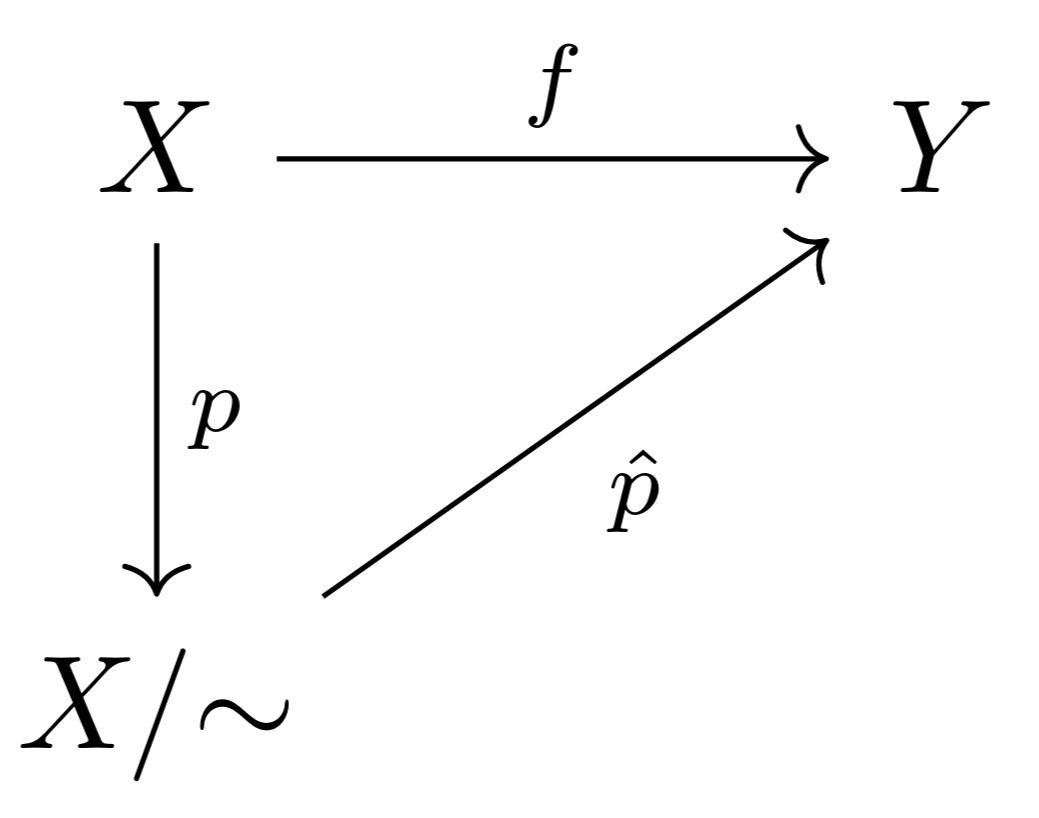
Proposition 2. Let $X$ be a topological space, and let $X / {\sim}$ be a quotient of $X$, with quotient map $p$. Let $Y$ be a topological space, and let $f \colon X \to Y$ be a continuous function which is constant on fibers, i.e., if $x$, $y \in X$ have the same image under the quotient map $p$, then $x$ and $y$ also have the same image under $f$. Then, there exists a unique continuous map $\hat{p}$ which makes the following diagram commute:

The idea behind this is that, given any point $x \in X$, since $f$ is constant on fibers, it only matters where the equivalence class $[x]$ under $\sim$ is sent by $f$, so $f$ ‘factors’ through the quotient space. But I won’t give a detailed proof of this here.

Now we can return to our original three spaces, $X$, $X / {\sim}$, and $S^1$. The quotient map $p \colon X \to X / {\sim}$ takes the form

In particular, the fibers are $\set{x}$ for $x \in (0, 1)$ and $\set{0, 1}$. Let $f \colon X \to S^1$ be the function $x \mapsto (\cos(2 \pi x), \sin (2 \pi x))$. This is certainly a continuous map, since both the functions $\cos$ and $\sin$ are continuous. I claim that $f$ is constant on fibers. To check this, I only need to look at the fiber $\set{0, 1}$, since all the others are singletons. Indeed,

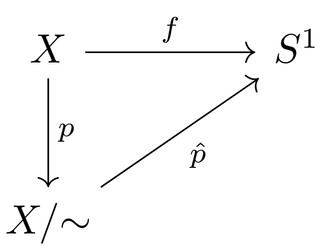
Since $f$ is continuous, and constant on fibers, the universal property of quotients asserts the existence of a unique continuous map $\hat{p}$ which makes the following diagram commute:

Now, the following is true about this picture:

• By the Heine-Borel theorem, $X = [0, 1]$ is compact, so the quotient $X / {\sim}$ is also compact, being the continuous image of compact space.
• $S^1$ is Hausdorff.
• $\hat{p}$ is a bijection, since every value of $\theta$ corresponding to a point on $S^1$ matches up to a unique fiber in $X / {\sim}$.

Hence, $\hat{p}$ is a continuous bijection from a compact space to a Hausdorff space, so $\hat{p}$ is a homeomorphism, by proposition 2. This shows that $X / {\sim} \cong S^1$, which establishes theorem 1.

This is the same argument used for more elaborate quotients, such as the torus, mentioned in the beginning.

• For all $a$, $b$, $c \in X$, if $a < b$ and $b < c$, then $a < c$ (transitivity)
• For all $a$, $b \in X$, exactly one of $a = b$, $a < b$, $b < a$ is true (trichotomy)

Say that $X$ is dense if for all $a$, $b \in X$ with $a < b$, there exists $c \in X$ such that $a < c < b$. Think $(\mathbb{R}, <)$, $(\mathbb{Q}, <)$ and $([0,1] , <)$, but not $(\mathbb{Z}, <)$.

Say that $X$ has no endpoints if for all $a \in X$, there exist $b$, $c \in X$ such that $b < a < c$. Think $(\mathbb{R}, <)$ and $(\mathbb{Z}, <)$, but not $(\mathbb{N}, <)$ or $([0, 1], <)$.

An example of a dense linear order with no endpoints is $(\mathbb{R}, <)$, but notice that this order is not countable. The countable, dense linear with no endpoints is $(\mathbb{Q}, <)$. Why the definite article? A remarkable fact about countable, dense linear orders without endpoints (that we proved as a tutorial problem in MT5861 Advanced Combinatorics at St Andrews) is that there is precisely one up to isomorphism.

Definition. If $(X, <)$ and $(Y, <)$ are linear orders, then a bijection $f \colon X \to Y$ is called an order isomorphism if for every $a$, $b \in X$ with $a < b$, we have $f(a) < f(b)$. Notice that, by trichotomy, there are no non-relations to be preserved, so being an order isomorphism is the same as being a bijective order homomorphism. We write $X \cong Y$ to denote order isomorphism.

Theorem. Let $X$ and $Y$ be countable, dense linear orders without endpoints. Then $X \cong Y$.

The proof of this is the original example of a so-called back-and-forth argument, used frequently in infinite combinatorics (another example being the random graph, which I think should instead be named the indestructible graph). This argument is due to Cantor.

Proof. Since $X$ and $Y$ are countable, we can enumerate them as $X = \set{a_0, a_1, a_2 \dots}$ and $Y = \set{b_0, b_1, b_2, \dots}$ (this enumeration definitely does not respect the orders). The idea is to inductively define an order isomorphism $f \colon X \to Y$ by adding an element of $X$ to the domain of $f$ at every even step, and adding an element of $Y$ to the image of $f$ at every odd step. This is the ‘back-and-forth,’ and is the reason we will be able to declare that the domain of $f$ is the whole of $X$, and the range of $f$ is the whole of $Y$. We will ‘feed’ our enumerations of $X$ and $Y$ into $f$, one element at a time.

Base case: Define $f_0 \colon \set{a_0} \to \set{b_0}$ by $f_0(a_0) = b_0$. This is an order isomorphism from $\set{a_0}$ to $\set{b_0}$ since there are no relations to check.

Inductive step: Assume that the isomorphism $f_k \colon A_k \to B_k$ has been constructed, where $A_k \subseteq X$, $B_k \subseteq Y$ are finite sets. The next step depends on whether $k$ is even or odd.

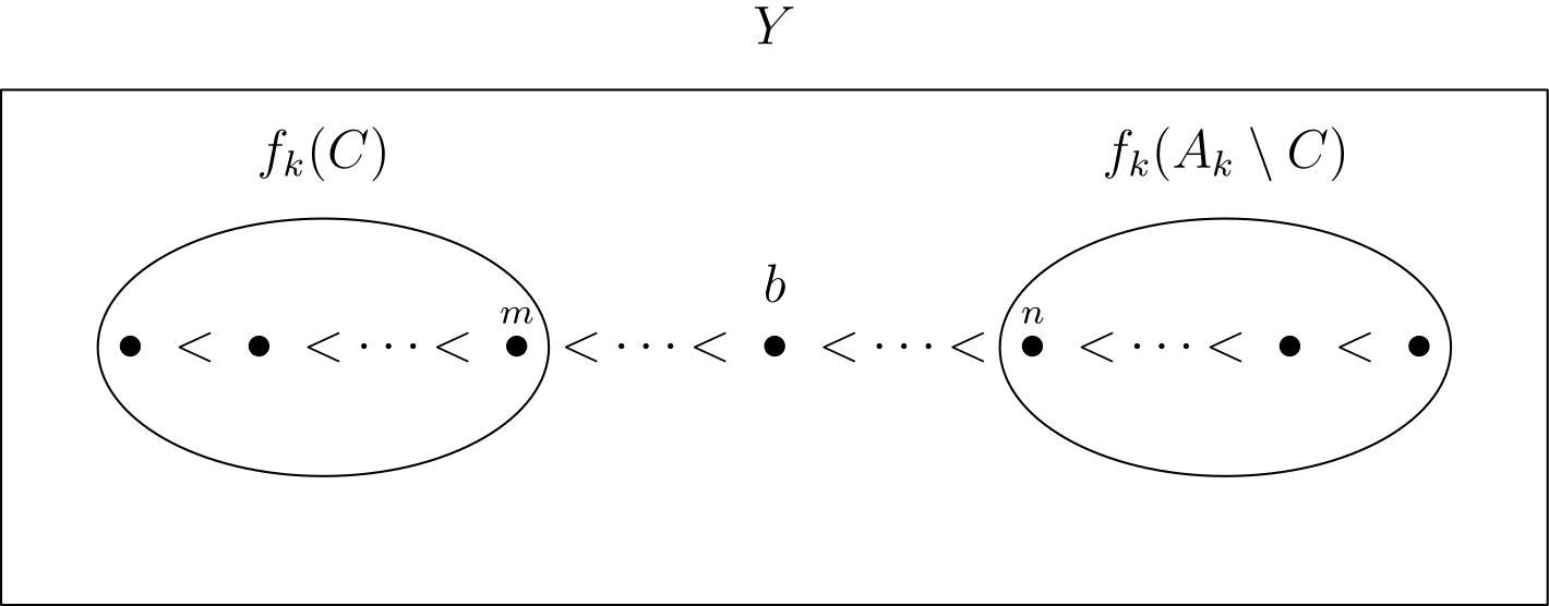
• Assume that $k$ is even. We will add the next element in our enumeration of $X$ which hasn’t yet been added to the domain of $f_k$. Let $a_i \in G$, where $i$ is the smallest natural number such that $a_i \notin A_k$. Define the set $C$ to be everything in $A_k$ which is less than $a_i$, that is $C = \set{c \in A_k \mid c < a_i}$ ($C$ may be empty, but this is accounted for). By trichotomy, (and since $a_i \notin A_k$), we can say that $A_k \setminus C = \set{ d \in A_k \mid a_i < d}$. Consider the sets $f_k(C)$ and $f_k(A_k \setminus C)$. Since $f_k$ is a bijection, these are disjoint, finite subsets of $B_k$ such that $B_k = f_k(C) \cup f_k(A_k \setminus C)$. We want to find $b \in Y$ such that $c < b < d$ for all $c \in f_k(C)$ and $d \in f_k(A_k \setminus C)$. Naturally, this depends on whether one of $f_k(C)$ or $f_k(A_k \setminus C)$ is empty, and this is where will be use both the assumptions of density and no endpoints.
  • Suppose that $f_k(C) = \emptyset$. Then $f_k(A_k \setminus C) = B_k$. Since $B_k$ is a finite linear order, it has a minimum element $n \in B_k$ such that, for all $d \in B_k$, we have either $n < d$ or $n = d$. Since $Y$ has no endpoints, there exists $b \in Y$ such that $b < n$. By transitivity, $b < d$ for all $d \in B_k$. This gives the desired $b$.
  • Suppose that $f_k(C) = B_k$, so $f_k(A_k \setminus C) = \emptyset$. This argument is dual to the previous one, using the endpoint condition on the other side. Since $B_k$ is a finite linear order, it has some maximum element $m \in B_k$ such that, for all $d \in B_k$, either $d < m$ or $d = m$. Since $Y$ has no endpoints, there exists $b \in Y$ such that $m < b$. By transitivity, $d < b$ for all $d \in B_k$. This gives the desired $b$.
  • Suppose that $f_k(C) \ne \emptyset$ and $f_k(C) \ne B_k$. Since $f_k(C)$ is a finite non-empty linear order, it has a maximal element $m \in f_k(C)$ such that, for all $c \in f_k(C)$, either $c < m$ or $c = m$. Similarly, since $f_k(A_k \setminus C)$ is a finite non-empty linear order, it has a minimal element $n \in f_k(A_k \setminus C)$ such that $n < d$ or $n = d$ for all $d \in f_k(A_k \setminus C)$. Since $Y$ is dense, there exists an element $b \in Y$ such that $m < b < n$. Then, by transitivity, we have $c < b < d$ for all $c \in f_k(C)$ and $d \in f_{k}(A_k \setminus C)$, as desired.

  
  

  

  
  

  Now that we have a suitable choice of $b$, we can define $f_{k+1} \colon A_k \cup \set{a_i} \to B_k \cup \set{b}$ by $f_{k+1}(a_i) = b$, and $f_{k+1}(a) = f_k(a)$ for all $a \in A_k$. By the inductive hypothesis, for any $a$, $a’ \in A_k$ with $a < a’$, we have $f_{k+1}(a) < f_{k+1}(a’)$. By the choice of $b$, for any $a \in A_k$ with $a < a_i$, we have $f_{k+1}(a) < f_{k+1}(a_i) = b$, and for any $a \in A_k$ with $a_i < a$, we have $b = f_{k+1}(a_i) < f_{k+1}(a)$. Therefore, $f_{k+1}$ is an order isomorphism, completeing the induction.

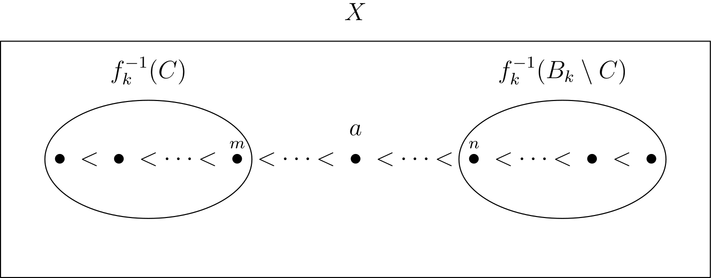
• Assume that $k$ is odd. Since $f_k$ is a bijection, it has an inverse $f_k^{-1}$. This lets us play the same argument that we used on the forth case on the back case. To that end, let $b_i \in Y$, where $i$ is the smallest natural number such that $b_i \notin B_k$. Define the set $C$ to be everything in $B_k$ which is less than $b_i$, that is $C = \set{c \in B_k \mid c < b_i}$. By trichotomy, (and since $b_i \notin B_k$), we can say that $B_k \setminus C = \set{ d \in B_k \mid b_i < d}$. Consider the sets $f_k^{-1}(C)$ and $f_k^{-1}(B_k \setminus C)$. Since $f_k$ is a bijection, $f_k^{-1}$ is a bijection, so these are disjoint, finite subsets of $A_k$ such that $A_k = f_k^{-1}(C) \cup f_k^{-1}(B_k \setminus C)$. Now, by the same argument used in the $k$ even case, we can find $a \in X$ such that $c < a < d$ for all $c \in f_k^{-1}(C)$ and $d \in f_k^{-1}(B_k \setminus C)$. This is where the density and no endpoints properties of $X$ are used.

  
  

  

  
  

  Defining $f_{k+1}$ the same way we did in the previous part, but with $f_{k+1}(a) = b_i$, we get an order isomorphism, completing the induction.

Now define

Since each $a_i \in X$ is accounted for at some even step in the induction, it follows that the domain of $f$ is the whole of $X$. Since every $b_i \in Y$ is accounted for at every odd step of the induction, it follows that the image of $f$ is the whole of $Y$. Since $f_i$ is an order isomorphism for every $i \in \mathbb{N}_0$, it follows that $f$ is an order isomorphism. Therefore, $X \cong Y$. $\square$

which is exactly what you might expect. In particular, you can show that this is the coarsest topology on $X \times Y$ which makes both projection maps continuous. That is, any other topology which makes both projection maps continuous has this one contained in it as a subset.

Things begin to go awry for an infinite product. For an indexed family of spaces $X_i$ for $i \in \mathcal{I}$, the product topology on the space $\prod_{i \in \mathcal{i}} X_i$ is defined to be the one generated by the basis

This all seems fine, apart from the condition that all but finitely many of the $U_i$ must be equal to the whole space $X_i$. This seems very arbitrary, and you may want to know why we can’t just define the topology to be the one with basis

and be done with it. This topology gets called the box topology on $\prod_{i \in \mathcal{I}} X_i$, and it contains the product topology as a subset, and is in most cases strictly finer than the product topology. For instance, if we take each $X_i$ to be a copy of $\mathbb{R}$ with the usual topology for $i \in \mathbb{N}$, then the set

is open with the box topology, but not with the product topology. So why is this a bad thing. To say why, we need to introduce a small amount of category theory. Informally, a category consists of a collection of objects, like groups, rings, vector spaces, or topological spaces, and morphisms between them, like group homomorphisms, ring homomorphisms, linear transformations and continuous maps. The morphisms are the structure-preserving maps between the objects. In category theory, we make definitions that only rely on the maps between objects, not on whatever is inside the objects themselves. Using this framework, we would like to make a wishlist of properties that we want the product space $\prod_{i \in \mathcal{I} } X_i$ to have. Most importantly, for each space $X_i$, we want the projection map $\pi_i$ onto $X_i$ to be continuous.

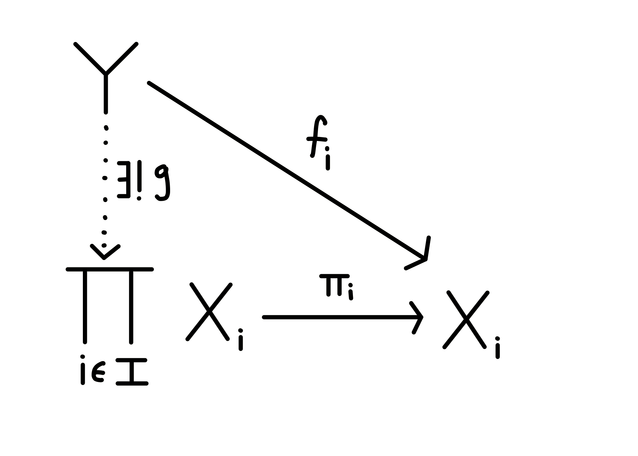
But this does not uniquely define the product topology on $\prod_{i \in \mathcal{I}} X_I$, since both the box and product topologies satisfy this property. What we need here is the idea of a universal property from category theory. If $\prod_{i \in \mathcal{I}} X_i$ is the product space with projection maps $\pi_i \colon \prod_{i \in \mathcal{I}} X_i \to X $, then for any other space $Y$ such that, for each $i \in \mathcal{I}$, there exists a continuous map $f_i \colon Y \to X_i$, we want there to be a unique continuous map $g \colon Y \to \prod_{i \in \mathcal{I}} X_i$ such that $f_i = \pi_i \circ g$.

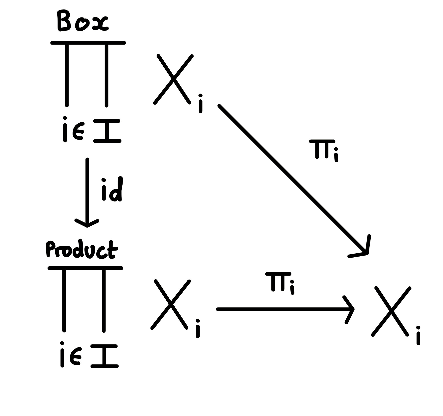
The above diagram is said to commute, when $f_i = \pi_i \circ g$. That is, we can factor every map from $Y$ into $X_i$ uniquely through the product space $\prod_{i \in \mathcal{I}}X_i$. For instance, with the box and product topologies on $\prod_{i \in \mathcal{I}}X_i$, the identity map makes the following diagram commute

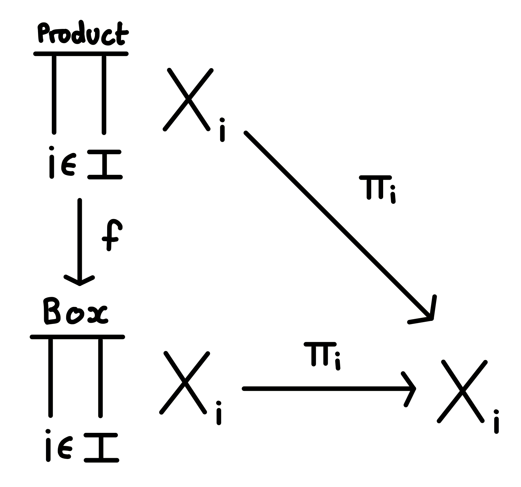
since every open set in the product topology is also open in the box topology. However, this does not work the other way around, since not every open set in the box topology is open in the product topology. To make things concrete, once again take each $X_i$ to be a copy of $\mathbb{R}$ with the usual topology for $i \in \mathbb{N}$. We want to find a map that makes the following diagram commute

To make the maps agree as functions, we must have $f$ as the identity map on the underlying set $\prod_{i \in \mathcal{I}} X_i$. But this map is not continuous, since the preimage of the open set

is itself, which is not an open set in the product topology, so we have been ripped away from the category of topological spaces. This shows that the box topology does not have the universal property of product. It can be shown that the product topology does indeed have the universal property of product, since it is the coarsest possible topology that makes the projection maps continuous.

An even more concrete way of showing that the box topology doesn’t make any sense is to once again look at our example of countably many copies of $\mathbb{R}$. We define the map

by $\tau(x) = (x, x, x, \dots)$. That is, $\tau$ is the diagonal map into $\prod_{i \in \mathcal{I}} X_i$. Its composition with the projection map $\pi_1$ is just the identity map on $X_1$, so $\tau$ is a very nicely behaved function. However, I claim that $\tau$ is not continuous in the box topology. Consider the set

$I$ is open in the box topology, but not in the product topology. The preimage of $I$ is $\tau^{-1} (I) = \set{0}$, which is not open in $\mathbb{R}$ with the usual topology, so $\tau$ is indeed not continuous in the box topology. This is clearly nonsense. You can check as an exercise that with the product topology, $\tau$ is actually a continuous function.

Theorem 1 Let $(X, d)$ and $(Y, d’)$ be a metric spaces, and let $f \colon X \to Y$ be a function. Then, $f$ is continuous if and only if, for every open set $U \subseteq Y$, the set $f^{-1}(U)$ is open in $X$.

Proof. $(\Rightarrow)$ Suppose that $f$ is continuous, and let $U \subset Y$ be open. Pick any $x_0 \in f^{-1}(U)$. Since $U$ is open, we can find $\epsilon > 0$ such that the open ball $B_{d’}(f(x_0), \epsilon) \subseteq U$. Plugging this value of $\epsilon$ into our continuity definition for $f$, we find that there exists $\delta > 0$ such that, if $x \in X$ with $d(x, x_0) < \delta$, then $d’(f(x), f(x_0)) < \epsilon$. Therefore, for any $x \in B_d(x_0, \delta)$, we have $f(x) \in B_{d’}(f(x_0, \epsilon) \subseteq U$. It follows that $x \in f^{-1}(U)$, and so, $B_d(x_0, \delta) \subseteq f^{-1}(U)$. Since $x_0$ was arbitrary, $f^{-1}(U)$ is open.

$(\Leftarrow)$ Now suppose that, for any open set $U \subseteq Y$, the set $f^{-1}(U)$ is open in $X$. Let $\epsilon > 0$ be fixed. For any $x_0 \in X$, the open ball $B_{d’}(f(x_0), \epsilon)$ is itself open in $Y$. Therefore, its preimage $f^{-1}(B_{d’}(f(x_0), \epsilon))$ is open in $X$, and so we can find $\delta > 0$ such that $B_{d}(x_0, \delta) \subseteq f^{-1}(B_{d_1}(f(x_0), \epsilon))$. In other words, $f(B_d(x_0, \delta)) \subseteq B_{d’}(f(x_0), \epsilon)$. We conclude that, for any $x \in X$ with $d(x, x_0) < \delta$, we have $d’(f(x), f(x_0)) < \epsilon$. Since $x_0$ and $\epsilon$ were both arbitrary, this means $f$ is continuous. $\blacksquare$

Now we will talk about what it means for two metrics to be equivalent. There are two different ideas here, one from analysis and one using topology. As we will see, one is stronger than the other.

Defintion. Let $(X, d)$ and $(X, d’)$ be metrics spaces. The metrics $d$ and $d’$ are called (bilipschitz) equivalent if there exist constants $0 < c_1 < c_2$ such that

for all $x, y \in X$.

Theorem 2. If metrics $d$ and $d’$ are equivalent, then they generate the same collection of open sets. That is, any set $U \subseteq X$ is open in $(X, d)$ if and only if it is open in $(X, d’)$.

Proof. Suppose that $d$ and $d’$ are equivalent. Let $U \subseteq X$ be open with respect to $d$, and pick any $x_0 \in U$. We can find $\epsilon > 0$ such that the open ball $B_d(x_0, \epsilon) \subseteq U$. Using the definiton of equivalence, for any $x \in X$ with $d’(x, x_0) < \epsilon / c_2$, we have

So, if $x \in B_{d’}(x_0, \epsilon / c_2)$, then $x \in B_d(x_0, \epsilon)$. It follows that $B_{d’}(x_0, \epsilon / c_2) \subseteq B_d(x_0, \epsilon) \subseteq U$. Since $x_0$ was arbitrary, we conclude that $U$ is also open with respect to $d’$. Since this situation is symmetric in the metrics $d$ and $d’$, the claim follows. $\blacksquare$

We might ask about the converse of Theorem 2.

Counterexample. Consider $\mathbb{Z}$ with $d_1$ the discrete metric, and $d_2$ the euclidean metric inherited from $\mathbb{R}$. Both of these metrics induce the same topology, namely the discrete topology, however they are certainly not equivalent metrics in the analytic sense: $d_1$ is bounded by $1$, and $d_2$ is unbounded.

Unlike the defintion of continuity, our definition of equivalence will not map over perfectly to topological spaces. This becomes a theme when making the jump from metric to topological spaces: many ideas from analysis gain a certain ‘fuzziness’ when brought over to topology, and we have to choose definitions that aren’t quite equivalent. We say that two metrics are topologically equivalent if they induce the same collection of open sets, which is a weaker notion that the analytic defintion. Another classic example of this fuzziness is the idea of limits of sequences in topological spaces.

Theorem 1 (Euclid-Euler) Let $a \in \mathbb{N}$ be even. Then $a$ is a perfect number if and only if $a$ can be written in the form $a = (2^{p-1}) (2^p - 1)$, where $2^p - 1$ is prime.

We begin by establishing a few basic facts about $\sigma$:

Claim 1 For any $p \in \mathbb{N}$, we have $p$ is prime if and only if $\sigma(p) = p + 1$.

Proof. If $p \in \mathbb{N}$ is prime, then the positive divisors of $p$ are precisely $1$ and $p$. It follows that $\sigma(p) = p + 1$. Conversely, if $p > 1$ is not prime, then $p$ has some positive divisor $1 < d < p$, so $\sigma(p) \ge 1 + p + d > 1 + p$. Finally $\sigma(1) = 1 \ne 1 + 1$, so we are done. $\blacksquare$

Claim 2 For any prime $p$ and $k \in \mathbb{N}$, we have

Proof. The set of positive divisors of the integer $p^k$ is precisely $\set{ p^a \mid 0 \le k \le a } = \set{1, p, p^2, \dots, p^k}$, so it follows that

as claimed. $\blacksquare$

Claim 3 For any coprime $a$, $b \in \mathbb{N}$, we have $\sigma(ab) = \sigma(a) \sigma(b)$; that is, $\sigma$ is a multiplicative function.

Proof. The idea is that, since $a$ and $b$ are coprime, each divisor of $ab$ can be expressed as the product of a divisor of $a$ and of a divisor of $b$ in exactly one way.

Let $a = p_1^{\alpha_1} p_2^{\alpha_2} \cdots p_n^{\alpha_n}$ be the prime factorisation of $a$, and let $b = q_1^{\beta_1} q_2^{\beta_2} \cdots q_m^{\beta_n}$ be the prime factorisation of $b$. Since $a$ and $b$ are coprime, none of the $p_i$ and $q_i$ are equal. Every divisor of $a$ is of the form $p_1^{x_1} p_2^{x_2} \cdots p_n^{x_n}$, where $0 \le x_i \le \alpha_i$. A similar observation is true of $b$. Conversely, every divisor of $ab$ is of the form $p_1^{x_1} p_2^{x_2} \cdots p_n^{x_n} q_1^{y_1} q_2^{y_2} \cdots q_m^{y_m}$, where $0 \le x_i \le \alpha_i$ and $0 \le y_i \le \beta_i$. The limits on $x_i$ and $y_i$ are true because $a$ and $b$ share no prime factors, so the largest power of $p_i$ dividing $ab$ is equal to the largest power of $p_i$ dividing $a$, and similarly for $b$.

By Uniqueness of Prime Factorisation, it follows that each divisor of $ab$ can be expressed uniquely as the product of a divsior of $a$ and a divisor of $b$; and conversely, if $d$ divides $a$ and $e$ divides $b$, then $de$ does indeed divide $ab$. This gives a natural bijective correspondence between divisors of $ab$, and products of a divisor of $a$ and a divisor of $b$.

Hence if the divisors of $a$ are $\set{d_1, \dots, d_k}$ and the divisors of $b$ are $\set{e_1, \dots, e_l}$, then $\sigma(a) = d_1 + \cdots + d_k$ and $\sigma(b) = e_1 + \cdots + e_l$, and

which is precisely $\sigma(a) \sigma(b)$. $\blacksquare$

Note: In Number Theory, a function $f : \mathbb{N} \to \mathbb{N}$ (or more generally to $\mathbb{C}$) is usually called multiplicative if it satisfies $f(ab) = f(a)f(b)$ for all coprime $a$ and $b$. If $f(ab) = f(a)f(b)$ for all $a$ and $b$ (not necessarily coprime) then $f$ is called completely multiplicative.

Note: Together, Claims 2 and 3 allow us to write down a complete characterisation of $\sigma(a)$ depending on the prime factorisation of $a$: if $a = p_1 ^{\alpha_1} \cdots p_k^{\alpha_k}$, then

While we won’t use this directly in the proof of Theorem 1, it’s nice to have.

Now, having collected these facts, we are in a good position to approach the proof of Theorem 1.

Proof of Theorem 1. We will first prove the converse, which was known by Euclid. We begin by supposing that $a = (2^{p-1})(2^p - 1)$, where $2^p - 1$ is prime. Since we want $a$ to be even, we may assume that $p \ge 2$. First, notice that $2^{p-1}$ and $2^p - 1$ are coprime: this is true since the only prime dividing $2^{p - 1}$ is $2$, meanwhile $2^p - 1$ is odd so has no factor of $2$. Therefore,

so $a$ is perfect.

The forward direction was not known by Euclid: it was proven by Euler in the 18th Century.

We begin by assuming that $a$ is an even perfect number. By the Fundamental Theorem of Arithmetic, we can write $a$ uniquely as $a = 2^k x$, for some natural number $k$ and odd number $x$. Since $x$ is odd, $2^k$ and $x$ are coprime, so $\sigma(a) = \sigma (2^k) \sigma(x) = (2^{k+1} - 1) \sigma(x)$ by Claims 2 and 3. Also, we assumed $a$ was perfect, so $\sigma(a) = 2a = 2^{k+1} x$.

It follows that

and so $\sigma(x) = 2^{k+1} y$, where

I claim that $y$ is an integer. Indeed, from the definition of $\sigma$, we know that

is an integer, so $2^{k+1} - 1$ divides $2^{k+1}x$. But $2^{k+1} - 1$ and $2^{k+1}$ are coprime, so $2^{k+1} - 1$ must in fact divide $x$. Hence $y$ is an integer.

By rearranging the definition of $y$, we have $x = y (2^{k+1} - 1)$, so $y$ is a divisor of $x$. Moreover, since $2^{k+1} - 1 > 1$ by the assumption that $k \ge 1$, it follows that $y < x$. Therefore, $\sigma(x) \ge x + y$.

Again from the definiton of $y$, we have $x = y (2^{k + 1} - 1) = 2^{k+1} y - y = \sigma(x) - y$, which leads us to $\sigma(x) = x + y$. Suppose for a contradiction that $y > 1$. Then $\sigma(x) \ge 1 + y + x > x + y$, which gives the contradiction we wanted. It follows that $y = 1$, and so $\sigma(x) = x + 1$, therefore $x$ is prime by Claim 1.

From this, it follows by setting $p = k - 1$ that $a$ can be written in the form $(2^{p-1})(2^p - 1)$, where $2^p - 1$ is prime, as claimed. $\blacksquare$

Famously, not much is known about odd perfect numbers. It is not even known whether they exist. It is also not known whether there are infinitely many perfect numbers: by virtue of the Euclid-Euler theorem, this is equivalent to knowing whether there are infinitely many Mersenne primes.

In general, $\sigma$ is a very interesting function to play around with, and has surprising links to many ideas in number theory. One can even reformulate the Riemann Hypothesis in terms of $\sigma$: the Riemann Hypothesis is equivalent to the statement that

for all $n \ge 5041$, where $\gamma$ is the Euler-Mascheroni constant. The above inequality is called Robin’s inequality.

So why study pure mathematics, if it is, by definition, mathematics which is not made with a real world use in mind? Many problems are not solvable without abstracting them, stripping away all of the unnecessary noise surrounding them, and focusing only on the important details. Pure mathematicians are interested in making abstract logical connections, sometimes with the hope that someone may one day come along and make real world use of their nice logic, and sometimes purely for the sake of making fuzzy ideas more precise.

As I said, my research is in graph theory. Graph theory occupies a place both in pure and applied mathematics: graphs are everywhere in fields like computer science, and are also fascinating mathematical objects of study for their own sake. I’m interested in the latter point, and specifically I’m studying pairs of ‘pseudo-similar’ vertices in graphs. These are vertices arising in pairs which posses an ‘almost symmetry’ which has frustrated efforts to prove a central conjecture in graph theory: the Graph Reconstruction Conjecture.

My research has focused on finding out how large a set of mutually pseudo-similar vertices can be packed into a graph of a given size. The way I’ve done this is rather peculiar: I’ve had to expand my definition of ‘symmetry’ in a graph to include far more things than I would traditionally call a symmetry. The first goal of my research was to reach a theorem classifying pseudo-similarity in terms of this ‘partial symmetry’. That goal has been completed, and now I’m trying to use my techniques to arrive at an answer as to exactly how many pseudo-similar vertices can be fit into a graph.

Something that stands out to me about completing a research project is just how much new mathematics I’ve learned over the course of my research so far, and how much this contrasts with the pace and style of a lecture course. This project has been the perfect opportunity to get to grips with some mathematical tools that I otherwise would have waited until the 5th year modules in Semigroups and Advanced Combinatorics to experience. Learning mathematics in order to apply it to research demands a much greater depth of understanding than to sit an exam, and I’ve enjoyed this change of pace very much.

However the research process has not always been smooth. A couple of weeks ago, I discovered that a theorem my supervisor and I thought was airtight actually contained a hole. After spending the past two weeks trying, and not succeeding, to patch this hole, I’m now realising that the story is probably much more complicated than we first thought. Unexpectedly, I’ve come to see this as a good thing. What was once a straightforward uniqueness theorem about pseudo-similar vertices in directed graphs has now turned into a string of quite useful lemmas about which partial symmetries of the graph can actually be extended to full symmetries. What I’m learning from this is that sometimes, messy and partial results tell a much bigger story than clean, complete results do. This gives an interesting contrast to the way mathematics is presented in our lecture notes.

So far, I’ve found the research process quite enthralling. Going into this project, I already thought I wanted to complete a PhD in mathematics, and this has definitely affirmed that ambition!